Fine Bubble Aeration System Design & Calculation: AOR/SOR Oxygen Demand, SOTE Efficiency, and Blower Sizing

In municipal wastewater treatment plants (WWTPs) and industrial wastewater biological treatment facilities, the aeration system serves as the core dynamic engine maintaining aerobic microbial metabolism and driving carbon oxidation and nitrification. Typically, the electrical energy consumption of the aeration system accounts for 50% to 70% of a plant's total operating electricity bill. During preliminary engineering design, errors in oxygen demand estimation, deviations in Standard Oxygen Transfer Efficiency (SOTE) values under actual mixed-liquor conditions, or miscalculations in blower discharge pressure versus piping headloss will cause severe operational failures: inadequate dissolved oxygen leading to sludge blackening, deflocculation, and effluent ammonia non-compliance; or severe over-aeration causing massive energy waste, hydraulic shearing of biological sludge flocs, and continuous off-design blower operation near surge thresholds.

This technical guide details the mathematical principles and hydrodynamic calculations behind fine bubble aeration system design. Moving beyond rough empirical "air-to-water ratio" estimations, we formulate the physicochemical conversion model from Actual Oxygen Requirement (AOR) to Standard Oxygen Requirement (SOR), quantify the relationship between diffuser placement density and SOTE, and provide a complete engineering calculation protocol for underwater air piping friction headloss and blower capacity matching.

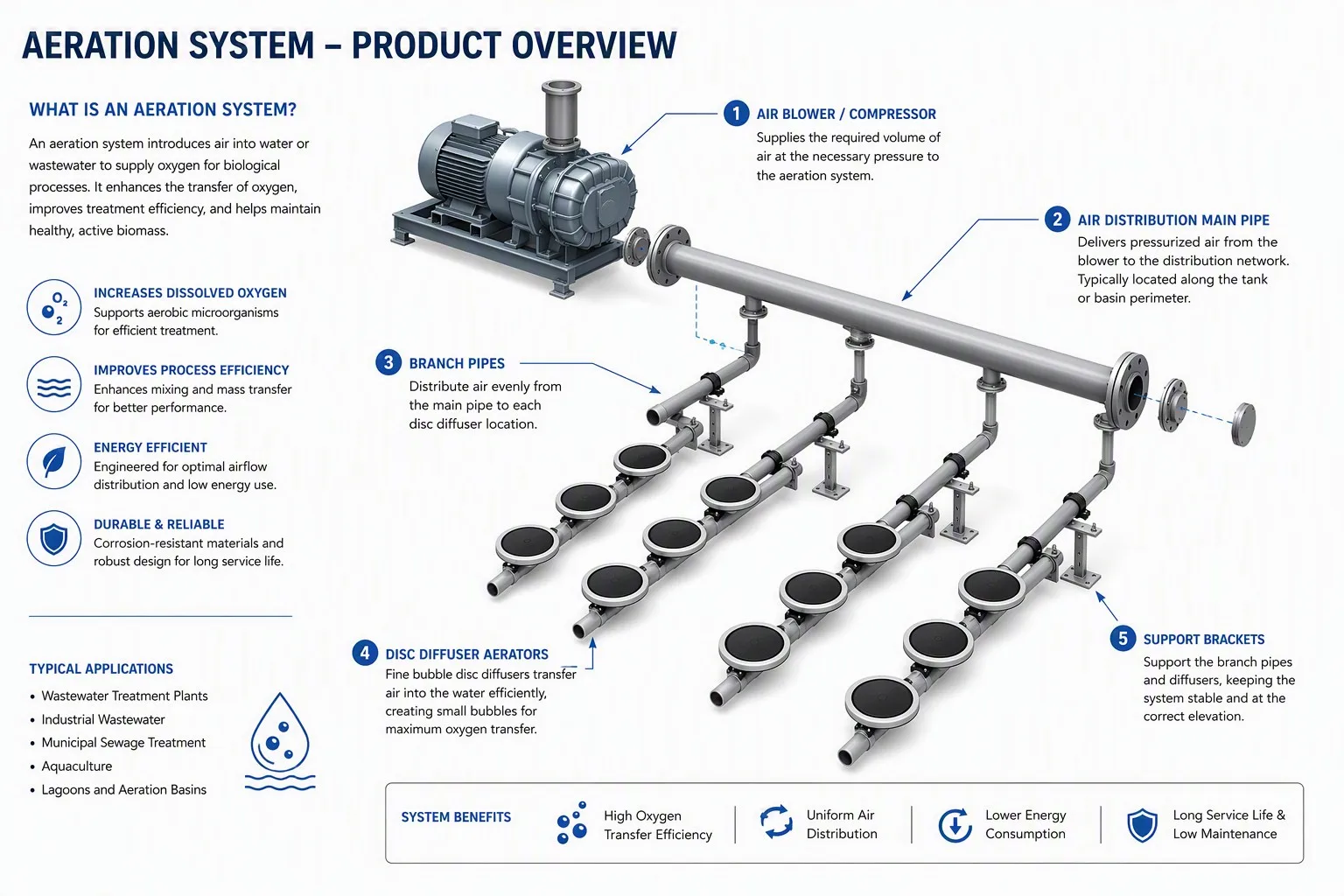
Figure 1: Fine Bubble Aeration System 3D Layout and Supply Air Piping Headloss Schematic

---

1. Oxygen Demand Calculations: Deriving SOR from AOR

The design of any aeration system begins with the metabolic oxygen requirements of the biological culture. In engineering practice, it is vital to distinguish between Actual Oxygen Requirement (AOR) under field wastewater conditions and Standard Oxygen Requirement (SOR) under baseline testing conditions.

1.1 Biological Actual Oxygen Requirement (AOR) Equation

Total biological oxygen demand in an aeration basin comprises carbonaceous BOD/COD oxidation, nitrification of ammonia nitrogen, endogenous cellular respiration, and the oxygen credit recovered through biological denitrification:

AOR = Q × [ a × (COD_in - COD_out) + b × (NH₄⁺-N_in - NH₄⁺-N_out) + c × V × MLVSS - d × ΔNO₃^--N ]

Standard engineering parameter guidelines (typical municipal wastewater):

• Carbonaceous Oxidation Coefficient (a): Typically 0.45 to 0.60 kg O₂ / kg COD removed.
• Nitrification Oxygen Coefficient (b): Theoretical oxidation of ammonia to nitrate requires 4.57 kg O₂ / kg NH₄⁺-N; accounting for cell synthesis, design practice applies 4.20 to 4.50 kg O₂ / kg N oxidized.
• Endogenous Respiration Rate (c): Typically 0.05 to 0.12 kg O₂ / (kg MLVSS·d), increasing significantly at elevated water temperatures.
• Denitrification Oxygen Credit (d): Nitrate reduction during anoxic denitrification returns approximately 2.86 kg O₂ equivalent per kg NO₃⁻-N reduced.

1.2 Converting AOR to Standard Oxygen Requirement (SOR)

Diffuser manufacturer ratings (such as clean water SOTE) are measured under standard laboratory conditions (water temperature T = 20°C, barometric pressure P₀ = 101.325 kPa, clean tap water, dissolved oxygen C = 0 mg/L). Conversion from field operating conditions uses the standard gas-liquid mass transfer equation:

SOR = AOR × [ C_s,20 / ( α × β × C_s,T,P - C_L ) ] × θ^{(20 - T)}

Key engineering correction factors:

• Apparent Oxygen Transfer Ratio (α): Wastewater surfactants, oils, and suspended solids hinder oxygen diffusion across the gas-liquid boundary. For municipal wastewater, α typically ranges from 0.80 to 0.88; in oily, hypersaline, or complex chemical industrial wastewaters, α frequently drops to 0.50 to 0.70.
• Saturation Correction Factor (β): Reflects the suppression of oxygen solubility caused by dissolved salts. For municipal effluent, β is 0.95 to 0.98; in high-salinity industrial wastewater, it may decline to 0.85–0.90.
• Temperature Coefficient (θ): Standard empirical constant for fine bubble diffused aeration is θ = 1.024.
• Design Operating DO (C_L): Aerobic basin setpoint, typically maintained at 1.5 to 2.0 mg/L.
• C_s,T,P: Oxygen saturation concentration at operating temperature T and effective mid-depth hydrostatic pressure P.

1.3 Practical Design Example: 20,000 m³/d Municipal WWTP Upgrade

Consider a municipal treatment facility with design influent flow Q = 20,000 m³/d, COD removal ΔCOD = 280 mg/L (0.28 kg/m³), ammonia oxidation ΔNH₄⁺-N = 32 mg/L (0.032 kg/m³), and denitrified nitrate utilization of 20 mg/L (0.02 kg/m³). Aerobic basin volume V = 8,000 m³, MLVSS = 3.0 g/L (3.0 kg/m³), design maximum summer water temperature T = 25°C, submerged water depth H = 6.0 m, and plant elevation = 200 m above sea level:

1. AOR Calculation:
   AOR = 20,000 × [ 0.5 × 0.28 + 4.3 × 0.032 - 2.86 × 0.02 ] + 0.08 × 8,000 × 3.0
   AOR = 4,412 + 1,920 = 6,332 kg O₂/d = 263.8 kg O₂/h.
2. Correction Factors & Solubility:
   With α = 0.85, β = 0.95, C_L = 2.0 mg/L, clean water saturation at 20°C C_s,20 = 9.17 mg/L, and effective mid-depth saturation at 25°C and 6.0 m depth C_s,25,P = 10.45 mg/L.
3. SOR Calculation:
   SOR = 263.8 × [ 9.17 / ( 0.85 × 0.95 × 10.45 - 2.0 ) ] × 1.024^{(20 - 25)}
   SOR = 263.8 × [ 9.17 / 6.438 ] × 0.888 = 333.6 kg O₂/h.

---

2. SOTE Efficiency, Diffuser Density, and Quantity Sizing

Once standard oxygen requirement (SOR) is established, the next design phase determines diffuser quantity, unit model selection, airflow capacity, and basin floor layout density.

2.1 Water Submergence Depth and SOTE Kinetics

Standard Oxygen Transfer Efficiency (SOTE) defines the mass percentage of oxygen absorbed by clean water relative to total oxygen supplied in the compressed air:

• Bubble Residence Time: Fine bubbles (1.0–2.0 mm diameter) ascend at an average terminal velocity of 0.25 to 0.35 m/s. Increased basin depth extends contact time between ascending bubbles and the liquid phase.
• Specific Transfer Rate: High-efficiency disc and tube diffusers generate an incremental SOTE of 6.0% to 8.0% per meter of effective submergence. At 6.0 meters submergence, overall system SOTE reaches 38% to 45%.

2.2 Diffuser Sizing and Quantity Calculation

Under standard ambient conditions, atmospheric air contains approximately 0.299 kg O₂ per cubic meter. Required standard air volume Q_air is calculated as:

Q_air = SOR / ( SOTE × 0.299 )   [Nm³/h]

Continuing the 20,000 m³/d example with a 6.0 m basin depth and SOTE = 40%:

Q_air = 333.6 / ( 0.40 × 0.299 ) = 2,789.3 Nm³/h ≈ 46.5 Nm³/min

• Option A: 12-Inch Disc Diffusers (Ø300 mm / Ø350 mm, e.g. AquaSust AS-DD270/AS-DD350)
  Standard design flux is 2.5–3.5 Nm³/h per unit (nominal 3.0 Nm³/h for optimal SOTE vs. headloss).
  Total diffusers required: N = 2,789.3 / 3.0 ≈ 930 units.
• Option B: Tube Diffusers (Ø63 × 1000 mm, e.g. AquaSust AS-TD63/AS-TD93)
  Standard design flux is 6.0–8.0 Nm³/h per 1-meter tube (nominal 7.0 Nm³/h).
  Total tube units required: N = 2,789.3 / 7.0 ≈ 398 units.

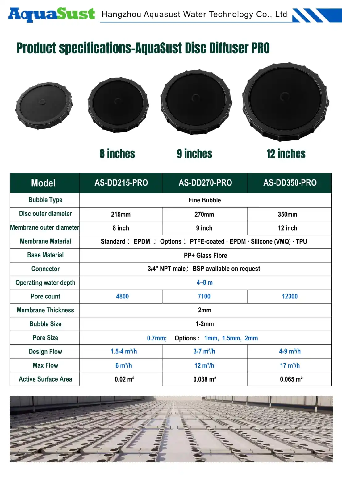
Figure 2: AquaSust High-SOTE Fine Bubble Disc Diffusers (AS-DD215, AS-DD270, AS-DD350)

2.3 Floor Coverage Rate and Anti-Coalescence Layout

Diffuser placement density must be carefully engineered to prevent dead zones while avoiding bubble coalescence:

• Floor Coverage Ratio (FCR): Defined as total active diffuser projected area divided by basin floor area. Optimum range is 8% to 20%.
• Bubble Coalescence Risk: If placement density exceeds 25%, adjacent bubble swarms collide and merge into coarse bubbles during their ascent. This dramatically reduces interfacial surface area, causing a 15% to 30% drop in actual SOTE.
• Layout Spacing Guidelines: Center-to-center disc spacing should be maintained at 500 to 800 mm. Lateral air branch pipe spacing is typically 800 to 1,200 mm, with a minimum 300 to 500 mm buffer distance from tank walls to avoid turbulent wall-friction disruption.

Figure 3: AquaSust PRO Fine Bubble Disc Diffusers with Wave-Groove Retaining Ring on PP Piping Aeration Grid

---

3. Blower Headloss and Operating Pressure Calculations

While required blower airflow capacity is defined by Q_air (adjusted for local intake temperature and barometric pressure), blower discharge pressure (head) must overcome total cumulative system hydraulic resistance.

3.1 System Headloss Equation

Total blower gauge pressure head at the outlet manifold combines five structural resistance components:

P_total = P_water + ΔP_membrane + ΔP_friction + ΔP_fittings + ΔP_margin

1. Static Liquid Head (P_water): Hydrostatic pressure from diffuser membrane surface to water level: P_water = ρ × g × H_submerged. At 6.0 m submergence, P_water = 1,000 × 9.81 × 6.0 = 58.86 kPa.
2. Membrane Dynamic Orifice Loss (ΔP_membrane): Resistance of elastomeric membrane micro-slits under design airflow. High-quality virgin EPDM or silicone membranes typically exhibit 2.5 to 4.5 kPa at nominal flux.
3. Pipe Friction Loss (ΔP_friction): Friction across stainless steel (SS304/SS316L) headers and distribution laterals. Designing within standard air velocities (main headers: 10–15 m/s, lateral branches: 4–6 m/s) maintains friction losses within 1.0 to 2.0 kPa.
4. Fittings and Valve Losses (ΔP_fittings): Minor dynamic losses from elbows, tees, reducers, and balancing butterfly valves. Standard engineering practice estimates this at 30%–50% of straight pipe friction, approximately 0.5 to 1.5 kPa.
5. Design Safety & Aging Margin (ΔP_margin): Accounts for long-term biofouling, scaling, and membrane elasticity aging over multi-year cycles. A design margin of 3.0 to 5.0 kPa is recommended.

Summing these components for the 6.0 m basin:

P_total = 58.86 + 3.5 + 1.5 + 1.0 + 4.0 = 68.86 kPa ≈ 0.69 bar (Gauge)

3.2 Blower Technology Selection Strategy

• Air Suspension / Mag-Bearing Single-Stage Turbo Blowers: Industry standard for high efficiency in large municipal WWTPs. Delivers polytropic efficiency of 75% to 82% with 40%–100% VFD turndown, generating 20% to 30% electricity savings compared to legacy rotary lobe blowers.
• Rotary Screw Compressors: Positive displacement geometry maintains high adiabatic efficiency under high discharge pressures (>70 kPa) and fluctuating flow requirements.
• Roots / Tri-Lobe Rotary Blowers: Cost-effective for smaller industrial plants with tight initial budgets, offering robust reliability despite higher noise and lower wire-to-air energy efficiency.

---

4. Reference Matrix: Key Diffuser Design Parameters

The following engineering reference matrix summarizes design standards and sizing values across common municipal and industrial applications:

Diffuser Model & Type	Target Wastewater Application	Design Flux per Unit (Nm³/h)	Membrane Headloss (kPa)	6.0m Clean SOTE (%)	Floor Coverage Rate	Aeration Efficiency (kg O₂/kWh)	Design Operating Life
9-Inch Disc Diffuser (Ø215 mm EPDM)	Medium/Small Municipal WWTP, Contact Oxidation	1.5 – 2.5 (Nominal 2.0)	2.5 – 3.8	36.0 – 40.0%	7% – 14%	4.2 – 5.8	6 – 8 Years
12-Inch Disc Diffuser (Ø300/350 mm EPDM)	Large Municipal WWTP, Basin Upgrades & Expansion	2.5 – 4.0 (Nominal 3.0)	2.8 – 4.2	38.0 – 43.0%	9% – 18%	4.5 – 6.2	6 – 8 Years
12-Inch Silicone Disc Diffuser (Ø300 mm)	Petrochemical, Oily Food, High-Temp Pharma Streams	2.5 – 4.5 (Nominal 3.2)	3.2 – 4.8	36.0 – 41.0%	8% – 16%	4.0 – 5.5	8 – 10 Years
Tube Diffuser (Ø63 × 1000 mm EPDM)	Plug-flow Channels, SBR, CASS, Narrow Basins	5.0 – 9.0 (Nominal 7.0)	3.0 – 4.5	37.0 – 42.0%	Pitch 0.8–1.2 m	4.3 – 5.9	6 – 8 Years
Retrievable Liftable Tube Grid	Zero-downtime Retrofits, Scaling/Hard Industrial Water	6.0 – 10.0 (Nominal 8.0)	3.5 – 5.2	35.0 – 39.0%	Modular Crane Frame	3.8 – 5.2	8 – 12 Years

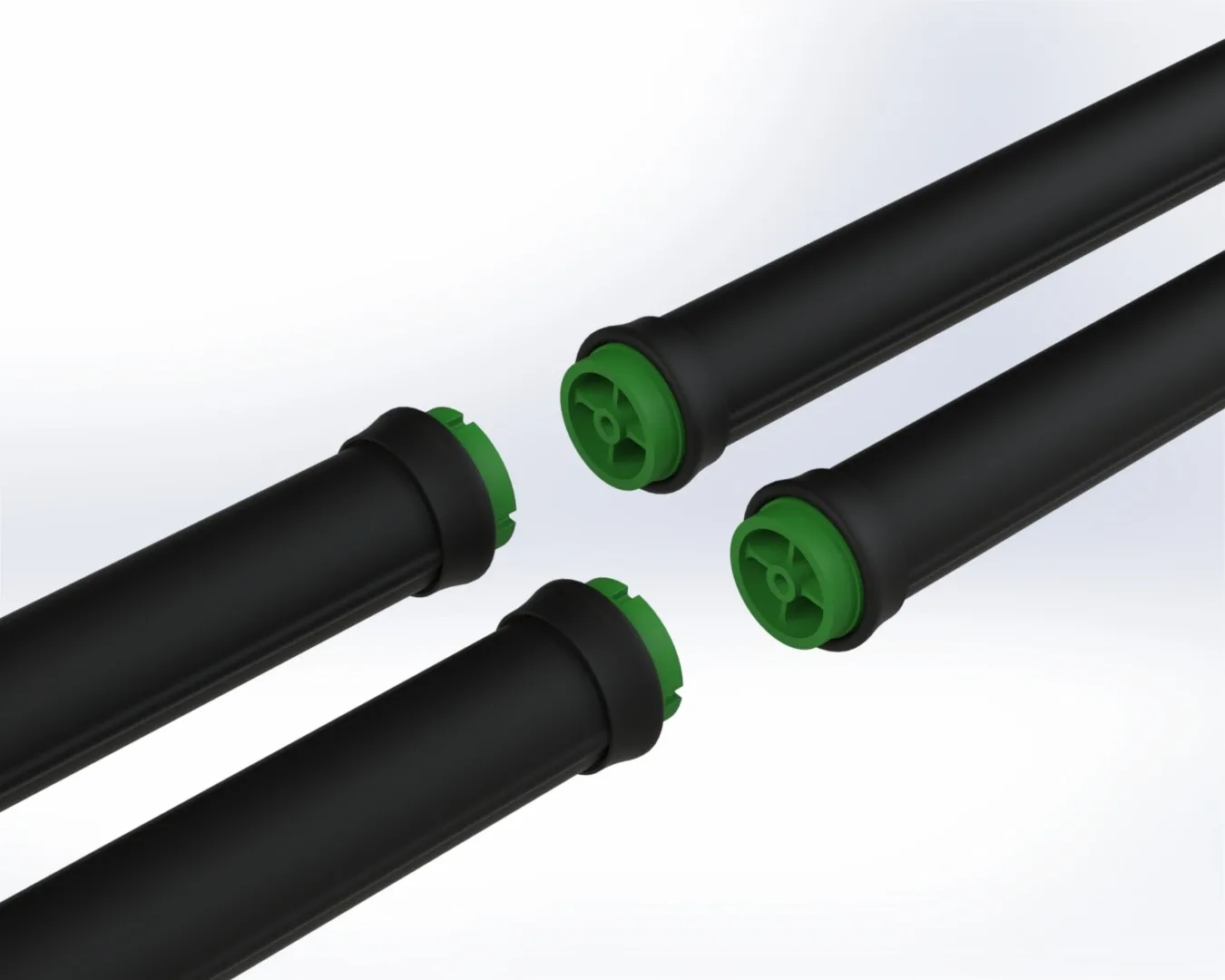
Figure 4: Retrievable Liftable Aeration Grid System Field Installation View

---

5. Environmental and Altitude Design Adjustments

Site altitude, ambient air pressure, and regional climate conditions directly alter blower air intake mass flow and oxygen solubility:

5.1 High Altitude Corrections

At elevated project sites (1,500 to 3,500 meters above sea level):

• Atmospheric pressure drops from 101.3 kPa at sea level to approximately 79.5 kPa at 2,000 meters, reducing air density by over 20%.
• To deliver the identical mass flow of oxygen (kg O₂/h), the blower inlet volumetric capacity (ACFM or m³/min) must be expanded by 15% to 30%, and hydrostatic saturation C_s,T,P must be recalculated.

5.2 Grid Frequency & Electrical Standards

• 50 Hz vs. 60 Hz: European, Asian, and Middle Eastern grids operate at 50 Hz (380–400 V), whereas North American and Latin American regions utilize 60 Hz (460–480 V).
• Direct-drive blower motors operating on 60 Hz run 20% faster than 50 Hz equivalents. Impeller sizing, dynamic balancing, and motor power curves must be verified to prevent motor overload.

5.3 Extreme Water Temperature Conditions

• Tropical Climates (30°C–38°C): Low dissolved oxygen saturation severely inflates SOR. Elastomeric membranes must use antioxidant-modified EPDM formulations to prevent thermal embrittlement.
• Cold Regions (5°C–10°C): Nitrification kinetics decline, necessitating longer sludge retention times (SRT) and larger tank volumes. Membrane elasticity at low temperatures must be checked against pressure loss spikes.

---

Frequently Asked Questions (FAQ)

Q1: How can engineers accurately determine the wastewater mass transfer coefficient α for complex industrial streams?

In industrial wastewater projects, assuming the municipal default of α = 0.85 can lead to severe oxygen deficits. The standard test protocol is the off-line non-steady-state re-aeration method. Fresh wastewater and demineralized water are tested under identical vertical column geometries and gas flow rates. The ratio of wastewater K_La to clean water K_La yields true α. Typical preliminary guidelines: Chemical/Pharma: 0.55–0.65; Textile/Paper: 0.60–0.70; Food/Beverage: 0.70–0.80.

Q2: If an existing basin suffers from bubble coalescence due to excessive diffuser density, what corrective actions can be taken?

1. Reduce Unit Airflow Flux: Use blower VFD control to lower per-diffuser airflow toward minimum operating thresholds (e.g. 2.0 Nm³/h on 12-inch discs), reducing bubble plume interaction.
2. Tapered Aeration Zoning: Modulate lateral valves to deliver tapered aeration: high airflow at the influent zone, transitioning to reduced airflow near effluent weirs.
3. Submersible Flow Boosters: Install low-speed horizontal flow makers above the diffuser grid. Horizontal cross-currents disperse ascending bubble plumes and prevent vertical bubble column fusion.

Q3: How do engineers prevent blower surge during low-load operations?

• Staged Blower Sizing: Configure multi-blower arrays with combinations of base-load and variable-load units (e.g. 2 duty + 1 standby) equipped with VFDs running safely between 45% and 100% capacity.
• Automated Blow-Off Anti-Surge Loops: Integrate PLC-managed blow-off valves linked to high-speed flow and pressure transmitters. When flow drops within 10% of the surge line, the valve modulates to maintain safe mass flow across the blower impeller.

---

Conclusion & Engineering Support

Fine bubble aeration design requires rigorous coordination of biochemical kinetics, gas-liquid mass transfer, and piping fluid dynamics. Precise AOR to SOR conversion, calibrated SOTE selection, and accurate system headloss modeling are critical to achieving compliant biological treatment while minimizing electrical power consumption.

As a global specialist in diffused aeration systems, AquaSust provides high-efficiency fine bubble disc diffusers (AS-DD series), tube diffusers (AS-TD series), plate diffusers, and custom liftable stainless steel aeration grids. Our engineering team provides complete aeration calculations, CFD basin modeling, piping loss audits, and equipment selection support to optimize your wastewater treatment infrastructure.